How to use Conditional Formatting in Excel?

Whether it is a slack message, email, or article, formatting is required to make the document more readable. Simple things like changing the font or bolding text can make a lot of difference to the document.

But when you are working in a spreadsheet, it may seem trivial to even spend time thinking about your formatting. If you learn how to use conditional formatting in excel online then, your spreadsheet will not only look good but you will also be able to do calculations speedy and efficiently.

What is Conditional Formatting?

As the name suggests, conditional formatting allows you to change the formatting of the spreadsheet depending on the rules that you have set. It provides you with more choices and control over icons and styles, better data bars, and the ability to highlight particular items in simple clicks.

Conditional formatting rule is made up of three parts:

Range: You begin by choosing the cells to which the rule will apply. It can anything, your complete spreadsheet or only a range of columns or rows.

Condition: It is about the “if” part of the if/then clause. You have various options to choose from, like less than, between, greater than, and more.

Formatting: It is the “then” part of the if/then clause. Excel online offers default styling for each condition but also provides the free option to customize it.
 

How to use Conditional Formatting in Excel?

There are several patterns of the formatting condition & styles, but the process is the same each time.

Let’s have a look at how to use conditional formatting in Excel:

• Choose a range.
• Click on the ‘Conditional Formatting’  under the Home section.
• Choose the rule (if needed, you can even customize the condition).
• Choose the formatting style.
• Now, click OK.

Choose a range

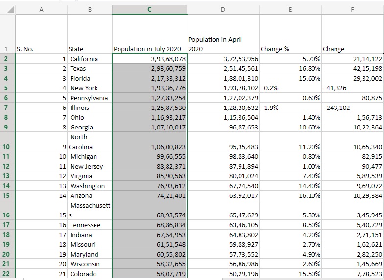
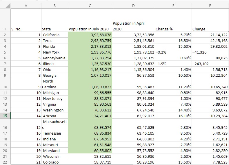
Before going to the ‘Conditional Formatting’ section, it is important to highlight the range of data you will be working on. The selection area can be anything, the entire spreadsheet, or just a specific column/row. For example, we have selected the C column here.
 Select the rule

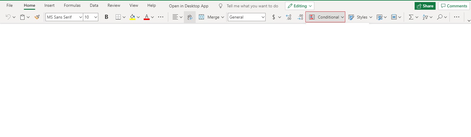
After the range is selected, click on the ‘Conditional Formatting’ option available at the top of the page.

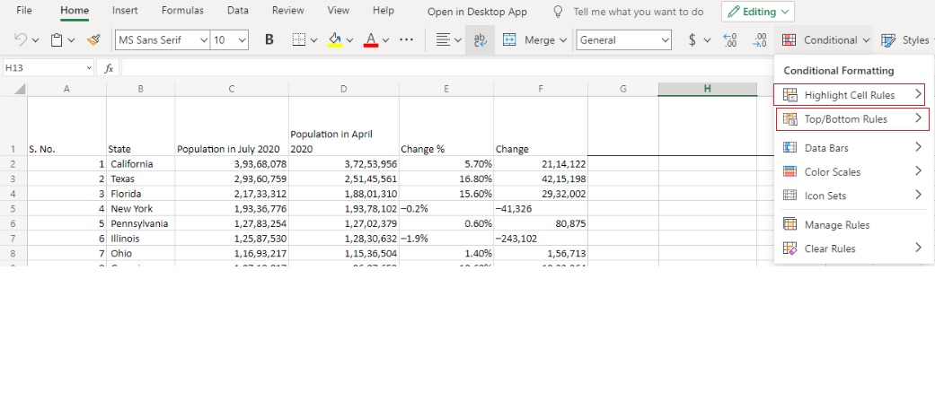
In the dropdown menu, you will view two basic rules: ‘Highlight Cell Rules’ and ‘Top/Bottom Rules.

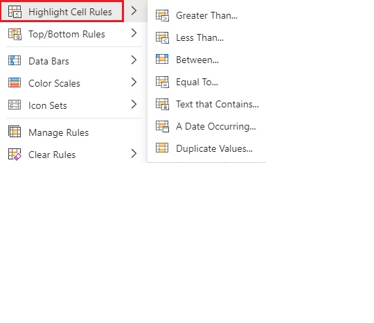
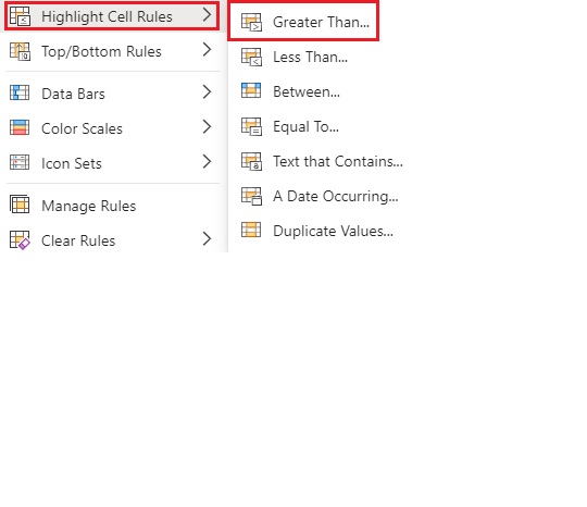
Under the ‘Highlight Cell Rules’ section, you will see the following options:

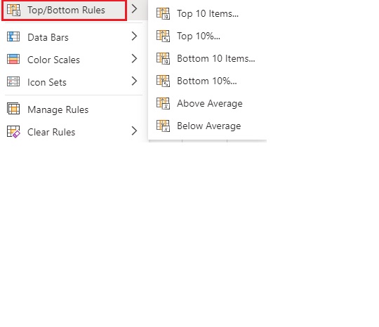
Under the ‘Top/Bottom Rules’ section, you will view the following options:

You can choose the rule meeting your needs. For example, here we have used the ‘Greater Than’ rule. You have to click on the ‘Highlight Cell Rules’ and then ‘Greater Than.

Select formatting

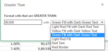
After choosing your condition, a formatting box will appear. On the left, you have to put value in the Format cells that are GREATER THAN box. For example, we have entered 60,000 to highlight the number of population in July 2020 in different states.

On the right side, you will have various options to choose from including:

• Light Red Fill with Dark Red Text
• Yellow Fill with Dark Yellow Text
• Green Fill with Dark Green Text
• Light Red Fill
• Red Text
• Red Border

These formatting options are common for all rules. Here, we have used Green Fill with Dark Green Text option to highlight.

Click on the ‘OK’ button and you will be able to view the important fields highlighted in the selected color.

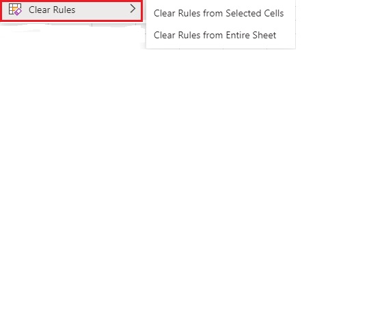
To clear the rules, click on Conditional Formatting> Clear Rules and then choose the ‘Clear Rules from Entire Sheet’ option. But if you just want to clear rules for a particular part then, click on the ‘Clear Rules from Selected Cells’ option.

Types of Formatting Rules and Styles

After learning about the conditional formatting rules, let’s learn about the other formatting options in Excel Online:

Highlight Cell Rules

The highlight cell rules like Greater Than, Less Than, Equal To, and Between are easy to understand & use. Here we will help you look at the other three options.

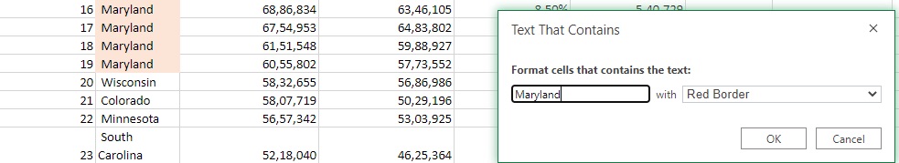
Text That Contains: This rule ‘Text That Contains’ will help you highlight cells that include specific text. It is helpful when you want to view how many times a name appears. For example, we have used this rule to distinguish Maryland.

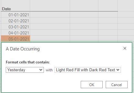
A Date Occurring : This ‘A Date Occuring’ is a dynamic rule where you can highlight cells that include the date from the previous week & month, next month & week, and so on.


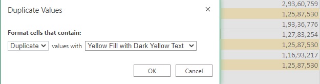
Duplicate Values: This rule helps to find duplicate as well as unique values. Choose the range and also select the rule, Duplicate or Unique you want to apply.

Top/Bottom Rules: This rule ‘Top/Bottom Rules’ helps in highlighting the worst and best performances from a chosen range with no math needed. You cannot customize the Above Average and Below Average rules, but you can customize the Top 10% and Top 10 rules.

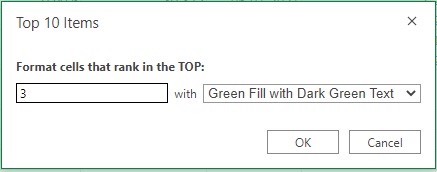
Enter the value in ‘Format cells that rank in the TOP’ so that you can highlight the Top 1 item, Top 5 items, or Top 100 items. For example, we have used this rule to highlight the top three states based on the population in July 2020.

Data Bars, Color Scales, and Icon Sets

The other three options in the Conditional Formatting section are completely visual.

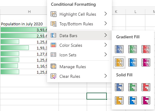
Data Bars in Excel Online makes it easy to view colorful bar graphs in a range of cells. A longer bar represents a higher value. You have to click on the Conditional Formatting and then Data Bars to view the data in bar graph format.

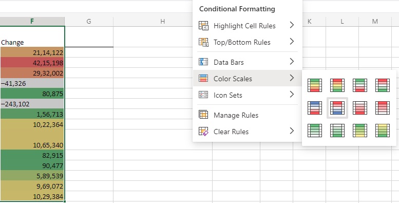
Color Scales provide a palette with different colored scales which you can apply to the cell selection. Depending on your choice and need, you can choose desired colored scales under the conditional formatting section and then clicking on the ‘Color Scales’.  Excel Online provides twelve different formats for color scales.

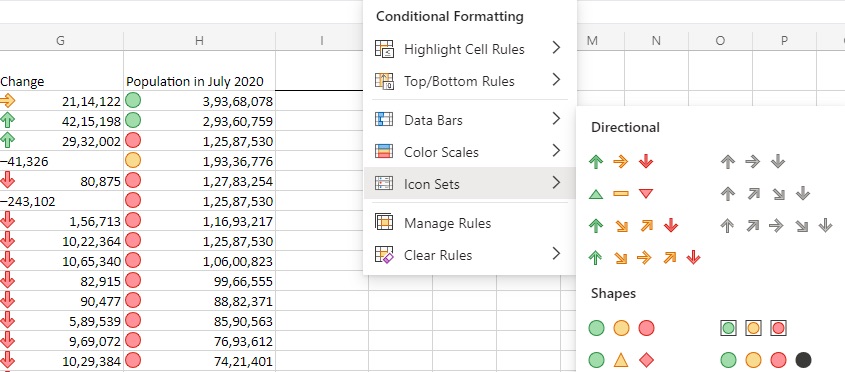
Icon Sets is available in the conditional formatting section and adds small icons at the edge of the cell.  Similar to the color scales feature, the icons are added depending on the numeric value. The icons will change when the values are edited.
Excel Online helps you to create spreadsheets from start or pick from different templates.  With the Appy Pie Connect and Excel integration, you can share your spreadsheets with other stakeholders & team members. Use Appy Pie Connect and integrate Excel Online with 150+ other apps to automate your business process in no time. It allows you to support queries into workflows, turn feedback into graphs, and more. Make the use of Excel Online to its maximum potential using Appy Pie Connect:

• Add calculations and formulas to bring your data to life and turn it into persuasive graphs & charts.  
• Invite others to collaborate to make easy progress on the projects.